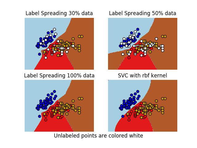
Decision boundary of label propagation versus SVM on the Iris dataset¶

print(__doc__)

# Authors: Clay Woolam <clay@woolam.org>
# License: BSD

import numpy as np
import matplotlib.pyplot as plt
from sklearn import datasets
from sklearn import svm
from sklearn.semi_supervised import label_propagation

rng = np.random.RandomState(0)

iris = datasets.load_iris()

X = iris.data[:, :2]
y = iris.target

# step size in the mesh
h = .02

y_30 = np.copy(y)
y_30[rng.rand(len(y)) < 0.3] = -1
y_50 = np.copy(y)
y_50[rng.rand(len(y)) < 0.5] = -1
# we create an instance of SVM and fit out data. We do not scale our
# data since we want to plot the support vectors
ls30 = (label_propagation.LabelSpreading().fit(X, y_30),
        y_30)
ls50 = (label_propagation.LabelSpreading().fit(X, y_50),
        y_50)
ls100 = (label_propagation.LabelSpreading().fit(X, y), y)
rbf_svc = (svm.SVC(kernel='rbf', gamma=.5).fit(X, y), y)

# create a mesh to plot in
x_min, x_max = X[:, 0].min() - 1, X[:, 0].max() + 1
y_min, y_max = X[:, 1].min() - 1, X[:, 1].max() + 1
xx, yy = np.meshgrid(np.arange(x_min, x_max, h),
                     np.arange(y_min, y_max, h))

# title for the plots
titles = ['Label Spreading 30% data',
          'Label Spreading 50% data',
          'Label Spreading 100% data',
          'SVC with rbf kernel']

color_map = {-1: (1, 1, 1), 0: (0, 0, .9), 1: (1, 0, 0), 2: (.8, .6, 0)}

for i, (clf, y_train) in enumerate((ls30, ls50, ls100, rbf_svc)):
    # Plot the decision boundary. For that, we will assign a color to each
    # point in the mesh [x_min, x_max]x[y_min, y_max].
    plt.subplot(2, 2, i + 1)
    Z = clf.predict(np.c_[xx.ravel(), yy.ravel()])

    # Put the result into a color plot
    Z = Z.reshape(xx.shape)
    plt.contourf(xx, yy, Z, cmap=plt.cm.Paired)
    plt.axis('off')

    # Plot also the training points
    colors = [color_map[y] for y in y_train]
    plt.scatter(X[:, 0], X[:, 1], c=colors, edgecolors='black')

    plt.title(titles[i])

plt.suptitle("Unlabeled points are colored white", y=0.1)
plt.show()