Note
Click here to download the full example code or run this example in your browser via Binder
Comparing various online solvers
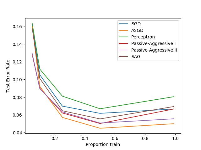
An example showing how different online solvers perform on the hand-written digits dataset.

Out:
training SGD
training ASGD
training Perceptron
training Passive-Aggressive I
training Passive-Aggressive II
training SAG
# Author: Rob Zinkov <rob at zinkov dot com>
# License: BSD 3 clause

import numpy as np
import matplotlib.pyplot as plt
from sklearn import datasets

from sklearn.model_selection import train_test_split
from sklearn.linear_model import SGDClassifier, Perceptron
from sklearn.linear_model import PassiveAggressiveClassifier
from sklearn.linear_model import LogisticRegression

heldout = [0.95, 0.90, 0.75, 0.50, 0.01]
rounds = 20
X, y = datasets.load_digits(return_X_y=True)

classifiers = [
    ("SGD", SGDClassifier(max_iter=100)),
    ("ASGD", SGDClassifier(average=True)),
    ("Perceptron", Perceptron()),
    ("Passive-Aggressive I", PassiveAggressiveClassifier(loss='hinge',
                                                         C=1.0, tol=1e-4)),
    ("Passive-Aggressive II", PassiveAggressiveClassifier(loss='squared_hinge',
                                                          C=1.0, tol=1e-4)),
    ("SAG", LogisticRegression(solver='sag', tol=1e-1, C=1.e4 / X.shape[0]))
]

xx = 1. - np.array(heldout)

for name, clf in classifiers:
    print("training %s" % name)
    rng = np.random.RandomState(42)
    yy = []
    for i in heldout:
        yy_ = []
        for r in range(rounds):
            X_train, X_test, y_train, y_test = \
                train_test_split(X, y, test_size=i, random_state=rng)
            clf.fit(X_train, y_train)
            y_pred = clf.predict(X_test)
            yy_.append(1 - np.mean(y_pred == y_test))
        yy.append(np.mean(yy_))
    plt.plot(xx, yy, label=name)

plt.legend(loc="upper right")
plt.xlabel("Proportion train")
plt.ylabel("Test Error Rate")
plt.show()
Total running time of the script: ( 0 minutes 14.029 seconds)
